LLM Benchmarking on the Nosana grid

Intro

The Nosana grid contains about two thousand nodes with various hardware configurations, which are actively running AI models. At the start of the Nosana test phase, these nodes have mostly been running image generation or transcription jobs through Stable Diffusion and Whisper. Although these jobs are suitable to make sure nodes are functioning properly, they do not provide any additional benefit from an AI use case perspective.

So to make the best use of the nodes until the launch of the mainnet, at the beginning of 2024 we started looking for opportunities to run jobs that would be useful to the Nosana community. As Large Language Models (LLMS) are projected to be the center pillar of Nosana’s AI demand in the foreseeable future, we decided to hire a dedicated AI specialist team to start working on a large-scale LLM Benchmarking project on the Nosana grid. This project aims to provide information that will help clients make better informed decisions, help the Nosana team implement a fairer market system, and contribute valuable information to the LLM research community. In this blogpost, we will go over the required fundamentals to understand how benchmarking works, and then show how we can use the results of the benchmarks to create fair markets.

LLM Fundamentals

Let’s start with the fundamentals of LLMs. What is an LLM? How does it work? And what do we need to run one?

Architecture

For anyone reading up on LLMs they might seem like complex neural networks used in artificial intelligence. While this is true to some extent, in practice, LLMs essentially consist of two easy to understand files. The model weights file, and the model code file. The model weights file contains the parameters of the model and determines the model size which is measured in bytes. The model code file contains the instructions on how to load and run the model.

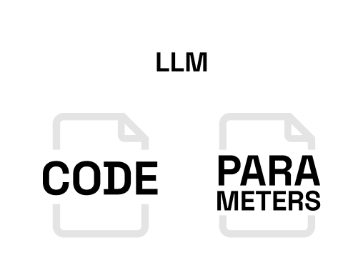
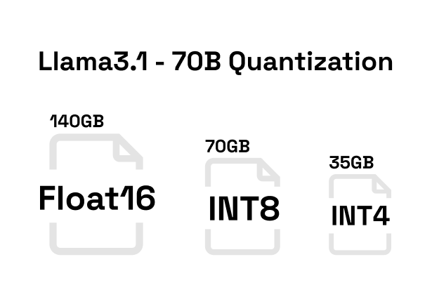
When looking at llama3.1–70B, the identifier 70B means the model contains 70 billion parameters. The parameters of the model are stored with 16-bit floating point precision, which equals to 2 bytes, making the model weights file size 140 gigabytes.

Each parameter in the model weights file corresponds to a neuron in the architecture described in the model code file. For most modern day LLMs this architecture is called a transformer. The image below shows a generalized transformer architecture used for producing text.

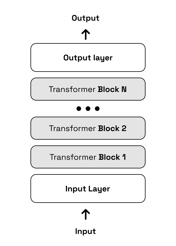
A detailed explanation of transformers is beyond the scope of this article, so we will focus only on the part that is the most important to understand for this benchmarking research. For a LLM to output text it needs to perform computations at every layer, and to do this, it needs to have its parameters and specific cached computations loaded into memory at the respective layers in the model.

Inference

Now that we know what an LLM is, let’s see how we actually produce language with them. LLMs are trained on the task of next token prediction. Tokens are units of text that correspond to words or parts of words, and they are the vocabulary that is understood by LLMs. So as far as LLMs are concerned, producing language is nothing more than correctly predicting the next word or subword given the preceding ones. This process of producing tokens with LLMs is called inference. The speed of inference is an important factor in the usability of LLMs, and it is influenced by the model size, architecture, and the hardware & software configuration on which it is run.

So how does inference work? To facilitate inference, LLMs go through 2 main stages. The prefill phase and the decoding phase.

In the prefill phase, the model processes all input tokens simultaneously to compute all the necessary information for generating subsequent tokens. In practice, the duration of this phase corresponds to the time you wait until the LLM starts generating its response. The prefill phase is highly parallelized and makes efficient use of the computing capacity, passing through the model only once.

At the start of the decoding phase, the model uses the cached information computed during the prefill phase to generate a token. From this point on, for every newly generated token, the previous token needs to pass through the network together with the cached computations. This process of repeatedly going through the network is not computationally intensive as computations only have to be performed for a single token. Instead, the decoding phase is memory intensive, because the cached information has to be moved around to perform the necessary computations.

The prefill phase is compute bound, while the decoding phase is memory bound. A process is considered compute-bound when it requires significant computation and its speed or performance is limited primarily by the amount of processing power of the hardware. A process is memory bound when its performance is limited by the rate at which data moves to and from memory. This rate is called the memory bandwidth.

Hardware Requirements

Alright, so we need compute and memory capacity to run LLMs. This is where our GPUs come in. Let's figure out what we would be able to run with the Nosana grid's most popular GPU, the RTX 4090. When considering GPUs, the available memory is expressed in VRAM, the memory bandwidth is expressed in bytes per second, and the computational capacity is expressed in FLOPS, floating point operations per second. The RTX 4090 has 24 GB VRAM, a memory bandwidth of 1,008 GB/s, and can produce 82.58 teraFLOPS.

The hard requirement for running an LLM is having enough VRAM to store its parameters + cached computations. For llama3–8B with 16-bit floating point precision, this would approximately be 18GB of VRAM. Our RTX 4090 will be able to handle that.

Figuring out if a model can be run is fairly straightforward, but figuring out how it will perform is hard to determine as it is dependent on many variables. That being said, given the constraint of a memory bound process we can give a rough theoretical estimation of the amount of tokens per second by dividing the model size by the memory bandwidth.

18GB ÷ 1,008 GB/s = 18ms

This calculation gives us 18ms per token or 56 tokens per second. So this calculation would give a rough estimation for an inference run with a single input sequence, which is a predominantly memory-bound process. However, if we would increase the amount of sequences processed at the same time, it could shift from memory-bound to compute-bound and the amount of FLOPS of the GPU would start to play a more important role.

Optimization

We have covered the fundamentals of LLMs and understand which variables are important for running them. By using optimization techniques we can tweak these variables resulting in beneficial tradeoffs that will allow us to run bigger models, or increase inference speed. There are many knobs to turn when it comes to optimization, but the three most important ones are quantization, computation enhancement and caching strategies.

Quantization reduces the precision of the model’s weights to lower bit representations. For example, if we would use quantization to transform the 16-bit floating point precision of our llama3.1–8B model to 8-bit integer, then we would reduce the model size from 16GB to 8GB. While this can have an impact on the accuracy of the model, the significant decrease in memory usage makes it a viable optimization technique.

Computation enhancement focuses on optimizing the operations performed within the model such as the attention mechanism. This mechanism is an important part of the transformer’s success, but also computationally expensive. By modifying the order of computations or by fusing together certain model layers we can reduce the data that needs to be written from and to memory.

Caching strategies involve the reduction of the cached computations that are kept in memory. By simplifying the structure of the cached computations it is possible to significantly reduce the memory footprint in exchange for a slight decrease in model accuracy.

Inference Frameworks

We have briefly gone over the main optimization techniques and it is already becoming apparent that implementing any potentially desired change might become complicated. Luckily, there are various LLM inference frameworks that provide an interface to a wide range of models with built-in options for optimization. As the field of LLM inference is rapidly evolving, these frameworks roll out updates frequently and there is no clear-cut best optimization framework.

One such framework is Ollama. We will give it a special mention here because it is the framework that was used to gather the initial benchmarking results. Ollama originated as a user-friendly framework with the goal of democratizing the use of LLMs. The Ollama team has impressively succeeded in achieving this goal, as it is undoubtedly the easiest framework for anyone with minimal hardware requirements to spin up an LLM. It is especially fitting for running and testing consumer grade hardware as its optimization techniques seamlessly allow models of any size to be run on GPUs with any amount of VRAM.

---

Nosana Benchmarking

Enough preliminaries. It is time to get into the actual benchmarking. Lets start off by going over the data we collected, and how we collected it.

Benchmarking Setup

As mentioned, Ollama was picked as the initial framework for benchmarking due to its compatibility with consumer grade hardware. With this framework in place, we implemented a custom made benchmarking script to gather data in two distinct categories, model performance and system specifications.

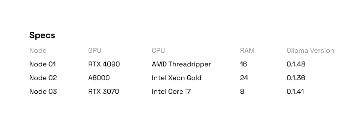
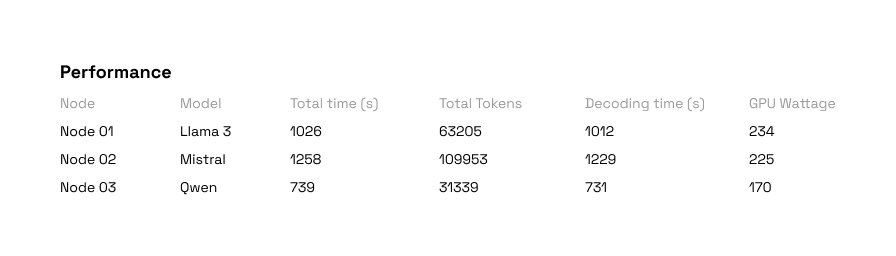
The performance data contains variables on the total amount of produced tokens and how long it took to produce them, but also the clockspeed and the wattage of the GPU. The system specifications data contains variables on an extensive set of system configurations that can have either large or small effects on model performance. The tables below illustrate the kinds of variables and their potential values.

With the to be collected variables defined, we now had to pick a model for benchmarking. Given the notable performance of the newly launched llama models and the Nosana nodes with a wide variety of VRAM capacities, we decided to pick llama3.1–8B that can fit on all GPUs.

Now for the actual procedure of benchmarking we had to create a method compatible with the current job posting structure of Nosana. A job has a maximum length of X hours, giving us plenty of time to load in one or more models, prompt them, and measure their performance. During a job every model got prompted with randomly sampled sequences such as “Write a step-by-step guide on how to bake a chocolate cake from scratch”. The content of a prompt does not have an influence on the performance of the model, but it does determine the length of the response, so to make sure the LLMs spent most of their time on actual inference the pool of prompts we made encouraged longer answers. At the end of each job the output contains the model performance and system specs variables which we extracted and added to a large dataset.

Evaluation

Before we get into the results, let's quickly look at the key evaluation metrics for LLM inference, inference speed and time to first token (TTFT). The inference speed is measured in tokens produced per second during the decoding phase, and largely determines how long a user has to wait for a full response. The TTFT is a measurement of the time a user has to wait for the first response token, which is a crucial component in the usability and desirability of many LLM applications.

In this first article, where we test consecutive single user queries, we will mainly focus on inference speed as a measure of performance, not the TFTT. The TTFT measurement is dependent on the pre-fill phase, which is a compute bound process as we mentioned. In our setting where we process single queries at a time, the amount of computations needed during the prefill phase is low, resulting in uniformly low TTFTs for all GPUs. Inference speed on the other hand, which is a measurement of how fast the decoding process is executed, is heavily dependent on memory bandwidth. There is a large variety of memory bandwidth capacity between the GPUs on the Nosana grid, so focusing on the inference speed metric will provide us with the most insightful observations.

As a final note on our evaluation procedure, it is worth mentioning that most LLM inference benchmarking research focuses on the hardware’s capacity to handle concurrent users. When dealing with concurrent users, the model has to handle multiple queries at the same time. This setting makes it possible to maximally utilize the GPUs memory and computational capacities, especially for enterprise hardware with large amounts of VRAM. We have deliberately chosen to perform this initial benchmark with consecutive single queries, or 1 concurrent user, to define a setting in which we can evaluate all GPUs on the Nosana grid. This makes it so that our results will help us identify well performing and underperforming nodes across all markets, which enables the implementation of a fair market structure. However, the current setup does not benchmark the actual maximum capabilities of the nodes, which will be a topic in one of our upcoming articles.

---

Results

The dataset we used contains information on 10,596 jobs performed by 550 unique nodes in 15 Nosana Markets. Within these nodes there are 39 unique types of GPUs. The RTX 4090 and 3090 are the most common GPUs by far with 122 and 101 counts respectively.

Market Performance

As an initial goal of our benchmarking research we set out to create fair markets. In the presented results we have aggregated the data on market level, so we can show the performance for each market and highlight opportunities for improvements.

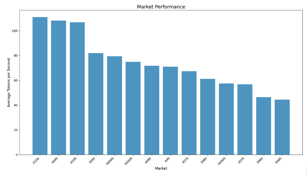
In the above visual we see the average tokens per second for each market. All the way at the top we have the H100 with 111 tokens per second, and at the bottom we have the RTX 4060 with 42 tokens per second. At first glance, this graph does not indicate anything out of the ordinary. On average the general trend seems to be, the more expensive the GPU the better the performance.

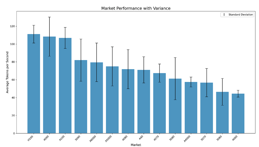
When we look at the performance variation within markets, indicated by the black bar, we get some more interesting findings. The larger the variation within a market the more varied the performance of different nodes within a market is. Varied performance within markets is undesirable for both clients and node runners. When clients use a Nosana node for inference compute, they want reliable performance suitable for their application. When node runners provide compute, they want to be paid based on the quality of compute they provide. A high variance within markets interferes with both of these objectives.

So having completely fair markets would mean that we would have a variance of 0 within all of them. However, getting to 0 variance within each market would require drastic solutions that impede the functionality of the Nosana grid. Fortunately though, designing the markets to minimize performance variance is something we can do. For example, we can implement a minimum performance threshold based on the average of each market. Every node performing worse than the average minus the performance threshold would be removed from the market. This would not only reduce the variance of the market, which is caused predominantly by underperforming nodes, but also increase the average tokens per second within the market.

The visual below illustrates what would happen to the market if a 20% or a stricter 10% threshold were to be implemented.

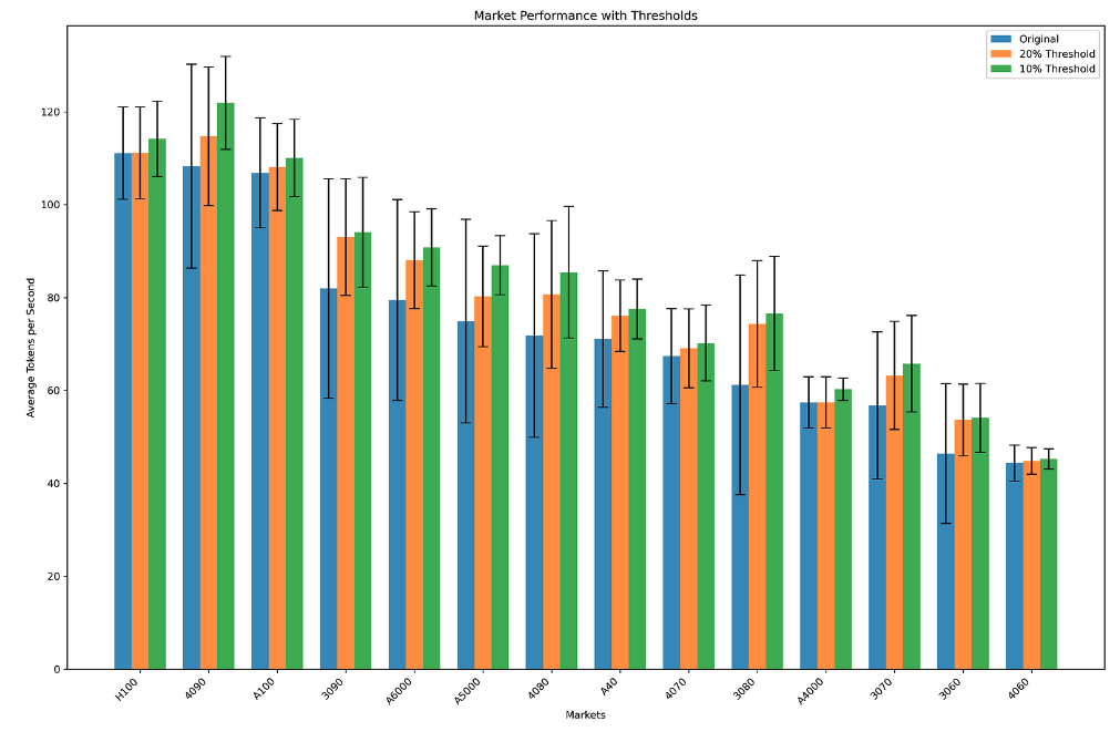
As we can see, for the markets with high variation, the threshold causes a significant increase in performance. This is because the threshold removes a larger amount of underperforming nodes within these markets. As a result, these markets become fairer because they provide more reliable compute to clients, and payout similar amounts for similar quality compute.

Performance Monitoring

After we observed the variance between nodes, we started analyzing variables that cause performance fluctuations. Even though we used a large set of hardware specs for our analysis, the results were unambiguous and pointed at two main factors responsible for performance, GPU type & Wattage. GPU type is the foundation that determines the performance range of nodes, but the wattage plays an arguably more crucial role by determining the location within this range. For example, a 3070 GPU running at full power can outperform a 4090 GPU that’s not getting enough, showing how proper wattage allocation can be just as important as the GPU model itself.

Now with this knowledge we are able to categorize 3 types of node runners that deviate from the expected performance. Spoofers, malignant node runners that fake hardware configurations & performance. Underclockers, economically greedy node runners that do not provide enough power to their hardware setup. And a third category of node runners with unforeseen technical issues. As the Nosana team we want to remove spoofers, keep underclockers in check, and help any node runner facing technical difficulties. Due to the unfakeable nature of model inference performance, monitoring this metric helps us identify which category of underperforming node runner we are dealing with, and take appropriate measures to balance the markets.

Node Leaderboard

As a first practical step towards fair markets we introduce the Nosana Node Leaderboard. Here we track the performance of each node within the market and display relevant hardware configurations. This allows us, together with the community, to monitor the performance of Nosana nodes in a transparent way. Go check it out!

---

Next Steps

By doing research using the Nosana Grid we aim to accomplish two main goals. First, to create the optimal Nosana experience by incorporating data-driven insights into our decision making. Second, to contribute valuable research findings to the broader large language model community. In this article we mainly focused on the first goal, as the current benchmark results are practically useful for the Nosana Grid, but do not provide information about the maximum performance capacity of specific model-hardware combinations in realistic settings. In our next article, we’ll explore maximum performance in real-world conditions.