LLM Benchmarking: Cost Efficient Performance

Economic viability is one of the most important factors in the success of new products and applications. No less so for Nosana. We show that the consumer-grade flagship RTX 4090 can provide LLM inference at a staggering 2.5X lower cost compared to the industry-standard enterprise A100 GPU.

Our previous article showed how we implemented a uniform LLM benchmark that helps track individual node performance and configurations. With this information, we are able to design fairer GPU compute markets by lowering their performance variation. But although the initial benchmark data is valuable in terms of market design optimization, it does not give meaningful insights into the realistic performance we are interested in. This is because the benchmark was designed to be compatible with all nodes on the network but it wasn’t able to test the full capacity of each node.

In this article, we address this limitation and zoom in on the performance comparison between consumer-grade and enterprise hardware. We implement benchmarks and use the results in a cost-adjusted performance analysis to highlight the competitive advantage of the Nosana Grid over traditional compute providers.

LLM Inference

When we talk about performance measurements in the context of LLM inference, we are mostly interested in inference speed. To better understand the factors influencing this speed, let’s begin with a brief overview of how LLM inference works.

The previous blog post went into more detail on this topic. If you have read it, you can skip ahead to this section. Readers who are interested in an in-depth explanation should refer to the previous blog post.

As far as computers are concerned, LLMs consist of two files. A large file containing the model parameters, and a smaller file that is able to run the model. The size of an LLM is determined by the amount of parameters it has and the precision of its parameters. Precision means the accuracy with which the model’s parameters are represented and is measured in bits. To calculate an example, let's take the popular LLM Llama 3.1 with 8 billion parameters and a commonly used 16-bit floating-point precision. One parameter with 16-bit floating point precision equals 2 bytes times 8 billion parameters, giving us a total model size of 16 GB. The model size is an important factor in the usability of LLMs because it determines which types of hardware are able to load the model.

Once loaded onto hardware, LLMs perform next-token prediction. This means that LLMs iteratively predict and add single tokens to an input sequence that is provided as context. This process of generating tokens is called inference. To perform inference, an LLM goes through two stages, the prefill phase and the decoding phase. During the prefill phase, the model processes all input tokens simultaneously to compute all the necessary information for generating subsequent tokens. During the decoding phase, the model uses the cached information computed during the prefill phase to generate new tokens.

In practice, the prefill phase corresponds to the time you have to wait until the LLM starts generating its response. It is a relatively short period that makes efficient use of available computing capacity through highly parallelized computations. We call the prefill phase compute-bound because it is limited by the computational capacity of the hardware running the LLM.

The decoding phase generally takes up the bulk of the inference time and corresponds to the period between the generation of the first and the completion of the last token. This process is not as computationally efficient as the prefill phase because it requires the constant on and offloading of cached computations between the processing units and memory. We call the decoding phase memory-bound because its performance is limited by how fast data can be moved to and from memory.

GPUs & Inference

In large production use cases, LLM inference is predominantly performed on high-end graphics processing units, or GPUs. Three key specifications of GPUs are particularly relevant to LLM inference:

1. VRAM (Video Random Access Memory): The amount of available memory on the GPU
2. FLOPS (Floating Point Operations Per Second): A measure of the GPU’s computational capacity
3. Memory bandwidth: The speed at which data can be transferred within the GPU

The processing of single sequences as described in the previous section usually leaves the VRAM and computational capacity of GPUs underutilized. To make better use of these resources we need to increase the amount of tokens processed and the computations performed. We can do this by processing a batch of multiple sequences at once. In production use cases this means that prompts from different users get bundled together and processed at the same time. Handling multiple requests, or concurrent users, plays an important role in the optimization of GPU usage.

Current Research

Alright, with the basics of LLM inference in mind, let's get more specific about the goal of the current research. Previously, we benchmarked the performance of all GPU types on the Nosana grid using Llama 3.1–8B with a single concurrent user. Running inference with a single concurrent user leads to GPU underutilization, limiting the insights gained when comparing performance with other compute providers. In this article, we set up benchmarks for accurate performance comparisons. We’ll focus our analysis on comparing Nosana’s performance against established cloud computing platforms. This comparison involves two key benchmarks:

• A baseline assessment measuring the performance of current market leaders
• An experimental evaluation of the Nosana grid’s performance

The Baseline Benchmark

Similar to running models on the Nosana grid, you can use a fully customized Docker image when renting a GPU from a compute provider. This means that we can keep important variables such as the model files and LLM serving framework constant for our experiment and only have to pick the GPU type and the price of usage for a fair comparison.

Because running LLMs in a production setting requires high capacity in terms of computation and memory, there are two main types to consider when renting a GPU, the A100 and the H100. The H100 is a newer and more powerful GPU than the A100, but both cards are able to load in and effectively run most open-source models. Given its relative affordability and arguable cost-effectiveness, we opt for the A100 as our baseline GPU.

For the price of usage variable there are more options to consider because there are various compute providers that offer a specific rental price per hour. To pick a competitive price we made use of the website https://getdeploying.com, which shows aggregated GPU rental prices for all cloud providers. At the time of writing the cheapest rental price for an A100–80GB is offered by Crusoe at $1.65 per hour, so we will use this price for our analysis.

The Experimental Benchmark

To compare the Nosana grid with our baseline approach, we need to determine the GPU type and an accompanying price per hour for our experimental benchmark. We’ll leave the price per hour as a variable to allow comparisons across multiple hypothetical pricing scenarios. This means that we only have to choose the GPU type.

The RTX 4090 is the most frequently encountered GPU on the Nosana grid, closely followed by the RTX 3090. The prevalence of the RTX 4090 and RTX 3090 GPUs on the Nosana grid highlights one of the network’s primary advantages over centralized compute providers: its ability to tap into a pool of underutilized consumer-grade hardware. Consequently, the most interesting comparison to make for Nosana is between popular enterprise hardware such as the A100 and underutilized consumer hardware such as the RTX 4090. Therefore, we pick the RTX 4090 for our experimental benchmark.

Research Setup

Let's go over the rest of the research setup. Now that we have determined the fixed variables for the baseline and the experimental condition, we have to pick the shared variables. The model, the LLM serving framework, and the number of concurrent users.

For the model, we picked Llama 3.1–8B. Llama models are the most used open-source LLMs in the world, and the 8 billion variant makes it possible to easily load the model on both the A100 and the RTX 4090 GPUs.

As an LLM serving framework, we experimented with both vLLM and LMdeploy. vLLM is one of the most popular frameworks and is frequently mentioned by our prospective clients. LMdeploy is a highly optimized framework and has shown the highest inference speed in recent benchmarking research. When using these frameworks, we used the out-of-the-gate inference configurations for both the baseline and experimental benchmark.

In our benchmarking script we implemented functionality to send concurrent user requests. While our previous article demonstrated that the 4090 slightly outperforms the A100 for a single concurrent user, this scenario rarely reflects optimized production environments. Therefore, we tested performance using 1, 5, 10, 50, and 100 concurrent users to see how the comparison holds up under different workloads.

As an evaluation metric, we used tokens produced per second, which directly measures inference speed. We evaluated both the A100 and RTX 4090 GPUs across all combinations of the variables mentioned above.

Results

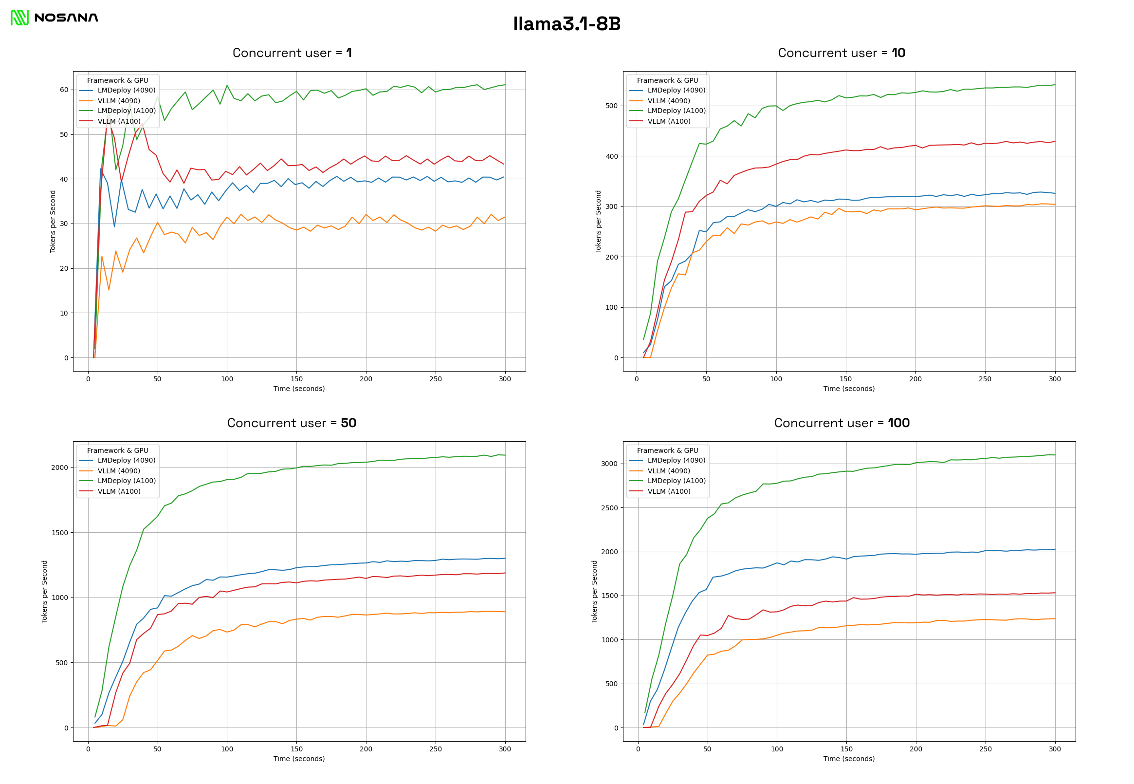
In the above graphs, we can see the performance of the RTX 4090 and the A100 with the LMdeploy and vLLM frameworks for different levels of concurrency. The graphs show that:

• At a low number of concurrent users, the A100s outperform the 4090s. However, this outperformance decreases relatively with the increase of concurrent users.
• At a higher number of concurrent users, LMdeploy greatly outperforms vLLM with its standard settings. The RTX 4090 with LMdeploy even outperforms the A100 with vLLM at 50 and 100 concurrent users.
• You need 1.5–2 RTX 4090s to reproduce the performance of an A100.

Price Comparison

Considering the respective purchase costs of the RTX 4090 and the A100, the performance results of the RTX 4090 are quite impressive. In this section, we analyze both GPUs’ performance while taking into account their purchase cost and operational expenses. For the cost-adjusted analysis we assume:

• The purchase cost of an RTX 4090 is $1,750.
• The purchase cost of an A100–80GB is $10,000.
• 2 RTX 4090s are required to reproduce the performance of an A100.
• The price of energy is equal to the average American price of $0.16 per kWh.
• The energy consumption of an RTX 4090 is 300W.
• The energy consumption of an A100 is 250W.
• The price for renting an A100 is $1.65.

Let’s start by calculating the return on investment (ROI) for the A100, which measures the amount of return relative to the investment cost. This helps us determine how quickly each GPU setup can earn its initial cost and start generating profit.

A100 ROI

1. Initial Investment: $10,000
2. Hourly Energy Cost: 0.25kW * 1 hour * $0.16/kWh = $0.04 per hour
3. Hourly Rental Revenue: $1.65 per hour
4. Hourly Net Profit: $1.65 — $0.04 = $1.61 per hour

To find the break-even point, we divide the initial investment of $10,000 by the hourly net profit of $1.61, which gives us approximately 6,211 hours or 259 days. Therefore, it would take about 259 days of continuous operation and rental to earn back the initial investment on the A100 GPU.

RTX 4090 ROI

Let’s perform a similar analysis for the RTX 4090 setup where we deliver the same performance as the A100 setup. Remember, we’re assuming that two RTX 4090s are required to match the performance of one A100.

1.  Initial Investment: $1,750 * 2 = $3,500
2.  Hourly Energy Cost: (0.3kW * 2) * 1 hour * $0.16/kWh = $0.096 per hour

Let’s first calculate the ROI assuming we rent out the RTX 4090 setup at the same price as the A100:

1.  Hourly Rental Revenue: $1.65 per hour
2.  Hourly Net Profit: $1.65 — $0.096 = $1.554 per hour

To find the break-even point: $3,500 / $1.554 per hour ≈ 2,252 hours or about 94 days

In this scenario, the RTX 4090 setup would break even much faster than the A100, in about 94 days compared to 259 days for the A100.

Now, let’s determine the hourly rental price that would allow the RTX 4090 setup to break even in the same timeframe as the A100. Here’s the calculation:

1. Hourly rate to cover initial investment: $3,500 / 6,211 hours = $0.56 per hour
2. Total hourly rate including energy cost: $0.563 + $0.096 = $0.66 per hour

This means that if we set the hourly rental price for the RTX 4090 setup at $0.66, it would break even at the same point as the A100.

Comparing this to the A100’s rental price of $1.65 per hour, we can see that the RTX 4090 setup could potentially be rented out 2.5X cheaper than the A100 while still achieving the same return on investment timeline. On top of that, the initial investment for the RTX 4090 setup is significantly lower than that of the A100, which reduces the barrier to entry for those looking to offer GPU rental services.

Wrapping Up

Through our comparison of the A100 and RTX 4090, we have demonstrated the potential competitive advantage that consumer-grade hardware has over enterprise hardware. As production models currently seem to trend toward smaller sizes, this benefit will only grow as more consumer-grade hardware becomes capable of running AI models efficiently. This trend holds enormous potential benefits for the Nosana grid, which primarily consists of consumer-grade technology.